Getting faster to decisions in A/B tests – part 2: misinterpretations and practical challenges of classical hypothesis testing

(this post is dedicated to Qixuan: thank you for all the patience on all the evenings I kept on bringing up various maddening questions, for the feedback on early drafts, and for all suggestions. This post wouldn’t be nearly as good if not for you!)

In the first post of the series, I covered some key approaches the industry uses to get to decisions faster than a classical null hypothesis testing approach allows. I also alluded that null hypothesis testing, while often highlighted for its basic statistical shortcomings (e.g., no peeking), has other pitfalls that are not immediately obvious.

In this post, I want to detail what I meant. In particular, I want to focus on practical challenges and easy-to-misinterpret concepts that are core to null hypothesis testing. I will not cover fallacies of p-values or issues in interpreting results – while they are confusing (here’s an academic paper that lists 25 (!) common misinterpretations), a lot of them come down to being pedantic and precise in communication. For the folks in the industry, there are more practical issues to consider.

A refresher on null hypothesis testing

Let’s begin with a quick recap of assessments of experiments using null hypothesis testing (NHT). Here is the process in a nutshell:

Before the test begins, we must decide how long an experiment will run. NHT does not allow multiple evaluations of ongoing results, so we have to set a cut-off time. Why exactly can’t we peek? Some great blog posts explain the reasons already, but it comes down to the fact that peeking reduces specificity (increases the risk of false positives). Even a few peeks can increase error rates to 3-4x the intended rate. I discuss some statistical solutions to this issue in the first post of the series.
The proper way to do it is by estimating the sample size required, which is a function of the certainty levels we want to achieve and the characteristics of the metric of interest. This is referred to as “power analysis”, and a bunch of calculators online help do the maths associating these factors, though it’s simple enough that you can easily code it up in a spreadsheet.
Once we have the sample size, we know the time it will take to run the experiment, and the experiment can begin.

Four factors express the certainty levels and the characteristics of the metric of interest:

Desired sensitivity level. This is also known as power or 1 – Type II error rate ( $1 - \beta$ ). It represents the true positive rate, i.e., the probability that the test will declare a difference between two variants when an actual difference exists between them. Usually, it is set to $1 - \beta = 0.8$ . The higher the sensitivity rate, the more data is required.
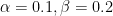
Desired specificity level, which represents the true negative rate. Typically, this is expressed as 1 – specificity, i.e., the error rate at which you declare variants in your experiment as different when they are the same. This is commonly referred to as the Type I error rate, a.k.a. statistical significance level $\alpha$ . The most common values used are $\alpha=0.05, 0.1$ . The higher the specificity level (the lower the error rate), the more data is required.
Minimum detectable effect (MDE) – the true effect size (difference in underlying populations) at which we want to achieve the specificity and sensitivity levels. Detecting a difference of 10% requires less data than detecting a difference of 1%. MDE typically depends on the expected impact of the change tested.
The variance of the metric. The more natural noise in the metric, the more data we need to differentiate the signal arising from the differences in the tested variants vs. the noise. In practice, variance is estimated using historical data of the metric of interest.

Now, let’s get into the challenges and misconceptions.

#1: How to choose specificity and sensitivity levels?

Statistics classes typically teach to use $\alpha=0.05$ as a default. Similarly, $\beta$ is usually set to $0.2$. Most software uses these default values, too, and I bet that most A/B tests in the industry do, too.

That is problematic. Should every business be 4x more concerned with false positives than false negatives by default? Is every experiment equal, and should these values be set in stone? Aren’t there some experiments where declaring an incorrect winner has limited business impact, but missing a difference may be more important? If not from a pure “did it move a metric” perspective, then from a team morale perspective?

Why do we use 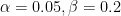$\alpha=0.05, \beta = 0.2$ ? It’s not that they are special. For an overview of how they came to be, I recommend this paper, but it comes down to the personal preferences of influential statisticians that, over time, became the standard. This is not a robust basis for decision-making.

On top, as I will show later, specificity and sensitivity may not even mean what you think they mean. Specifically, they do not represent long-term error rates that you can expect to make across multiple experiments – which is a very intuitive way to think about them.

Are there alternatives that do not require thinking about sensitivity and specificity levels? Yes and no.

A surface answer is that Bayesian methods don’t rely on these exact concepts. However, there is no way to get away from quantifying uncertainty, and even Bayesian methods require some decisions about sensitivity and specificity levels. However, the way they go about it may be more intuitive, partly because it becomes part of interpreting results rather than being a discussion before the experiment even begins.

#2: How to choose MDE?

Challenge #1 is conceptual; most teams will likely “solve” it using default values. This challenge is more practical, something that product managers and data analysts actually think about. How do you choose the right MDE?

MDE represents the hypothesized true underlying difference in populations. So, conceptually, one should pick an MDE corresponding to the expected impact of the tested feature. But how do you reason about it? How do you decide if it should be 1% or 0.8% for a given feature? What about 0.5%? You could, in theory, use the track record of past experiments and knowledge of a given feature to guide MDE selection, but it’s really hard. After all, we run A/B tests precisely because we do not have a good gut feeling about the impact of the feature. If we knew it, there would be no need to test.

It does not help that MDE is, in practice, the only adjustable parameter in sample size determination. If touching error rates is out of the question, then one way to get results faster is by assuming a higher MDE. To make matters worse, the relationship between MDE and the sample size is non-linear. For example, a test with 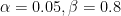$\alpha=0.05, \beta=0.8$ , where the expected conversion rate is 50%, an MDE of 2% will require ~10,000 observations in each variant. To detect 1% MDE, the sample size increases 4x. That may be a difference between running an experiment for a week vs. a month! There is a huge incentive to “pick” a higher MDE.

Choosing MDE is hard even if you can resist that incentive and stick to MDE as it should be thought about: the hypothesized difference in populations.

In practice, however, MDE is often misinterpreted as “impact we will be able to detect”, which further compounds the issue. Partly, I blame the very unintuitive MDE definition, which, I think, deserves a separate heading.

#3: What does MDE even mean?

A situation in the first post in this series illustrates a common misconception of what MDE means:

A product manager asks: “soo.. we always use a power level of 80%, and we ran these past five experiments with ~10,000 users each, and that implied a minimum detectable effect of 1.5% on our key metric.. but we detected an effect of 0.8% on two of them. How come? I thought the point of minimum detectable effect was that it’s a minimum change we can detect, but we seem to be able to detect lower changes, too?”
(this actually happened to me in real life)

I would not blame the product manager! My perspective of what MDE represents changed a lot while writing this post, too (and resulted in most redrafting..). Even when looking at first search results from the web, it “feels like” MDE has to do with the results you observe:

The minimum detectable effect (MDE) is the effect size which, if it truly exists, can be detected with a given probability with a statistical test of a certain significance level.
Analytics-toolkit.com

Minimum detectable effect (MDE) is a calculation that estimates the smallest improvement you are willing to be able to detect. It determines how “sensitive” an experiment is.
Optimizely.com

I think one should be excused to conclude that MDE is the smallest difference between two samples that produce p-values low enough to reject the null hypothesis. Or in other words, “MDE is the size of observed effect I can expect to detect with chosen error rates and given the sample size required”.

Except it’s not.

MDE has (almost) nothing to do with the sample differences you will observe. It’s an input parameter of your assumed true population differences to sample size/power calculations. The output of those calculations guarantees that you will reject a null hypothesis of no differences based on observed samples at selected error rates. Not a null hypothesis of differences larger than MDE; just a difference of zero (that is the answer to the product manager’s question).

This is not to say that MDE is useless. It forces you to make an assumption about the difference in underlying populations – exactly what you should be concerned with, instead of just the observed sample data. But given MDE may be the only “tunable parameter”, it’s easy for discussions about MDE to become more about “what impact we could detect” and not “what underlying impact we hypothesize.”

This line of thinking is very wrong. MDE should not be tunable to achieve statistical power levels – it’s like putting a carriage in front of a horse. Assuming a higher MDE for a low-impact feature doesn’t increase power. You cannot trade off MDE against sample size. The only choice available is sample size vs. power, not sample size vs. MDE.

Wouldn’t it be nice if there was an alternative that does not use this subject-to-abuse concept? Again, some Bayesian approaches (specifically, the expected loss metric) provide alternatives.

Bonus question

Is this whole MDE business clear to you? How about a bonus question?

Suppose you observe a statistically significant difference of 0.2 (e.g., p-value 0.04) in a typical experimental setup using an MDE of 0.5. How do we report results?

On the one hand, we observe a difference of 0.2, a p-value below our threshold, so we reject the null. We do not accept any alternative hypothesis – we just reject the one that they are equal. On the other hand, our sample size was set up in a way that should give this result 80% of the time for one particular alternative hypothesis (differences are at least 0.5).

So.. what is the effect you should report to the CEO? 0.2, the observed one? Or 0.5, which may be the true underlying effect? Could you say “we observed a difference of 0.2, there’s a 5% chance the result is by chance, and an 80% chance that the true difference is at least 0.5”?

Could you?

🤔

This brings me to the next point.

(the answer is – no; you can’t really report based on MDE. The 80% is the probability of observing the result given the alternative hypothesis; it’s not the probability of the alternative hypothesis given the result)

#4: NHT results are presented as binary

This challenge is of no fault of the statistical procedure itself but an important one to discuss. Most of the time, A/B test results are presented as binary: they are either (statistically) significant or not. If they are, the effect size is added (“feature X increased conversion by 0.5%”).

This sort of presentation hides the additional information we get from NHT – the statistical uncertainty. You may say – but what about confidence intervals? Sure, they may be used by some teams. But, likely, even when they are, they are only used when the effect is deemed statistically significant, to begin with.

In effect, thus, A/B test outcomes are binary. We either get enough evidence to reject the null hypothesis (typically, at a very high standard – allowing only a 5% error rate), or we don’t. This approach makes sense in, for example, a new drug research setting – the drug either works or does not. You want to be certain that one or the other is true.

But in a typical A/B test setting? Would it not be better to qualify a statement about outcomes with a certainty element? “we are 40% sure this variant increases conversions” or, even better, “we are 30% sure that this variant increases conversions by at least 1ppt; there also is a 15% chance it reduces conversions”.

One may say: sure, you can do that with NHT. Just show wider confidence intervals; 70%, 80% ones! Indeed, one could do that. My argument is not about statistics. It’s about the fact that, in practice, NHT usage withholds critical information from decision-makers. These people are paid to make the right decisions, and they should be able to make these choices with more information than the “significant or not” binary outcome of a test.

There is, however, a statistical element to it, too. NHT outcomes cannot be directly interpreted as probabilities. The confidence interval definition is weird, too. And then there’s the MDE business discussed above. This is where Bayesian methods again take the spot – interpreting results is more intuitive.

We’re left with just one more thing to cover, but it will take a bit more work and code to get through. Feel free to take a break!

#5: α and β are not long-term error rates

I glanced over one important aspect of sensitivity & specificity definitions earlier. They represent rates of avoiding errors. But rates over what, exactly?

Well, NHT is a procedure from frequentist statistics, and frequentist statistics are built on the concept of using samples to make inferences about the entire population. Correspondingly, these error rates reflect the probability of making an inference mistake purely due to the sampling error. The probability that we will get “unlucky” with a random draw from a population.

It’s easiest to illustrate with some simulations. Here is the setup:

Two variants: A (control) and B (treatment)
Decision metric: conversion rate (mean of a binary outcome variable)
Current conversion rate: 42%
Error rates: $\alpha=0.1, \beta=0.2$
We are comfortable with the minimum detectable effect (MDE) of 2ppt (i.e., we want to detect when the conversion rate of variant B drops below 40% or increases above 44%).

Plugging the above parameters into a power calculator yields a sample size of ~7,600 observations in each variant.

#setup
alpha = 0.1
power = 0.8
baseline_conversion_rate = 0.42
minimum_detectable_effect = 0.02
power_calcs = power.prop.test(
  p1=baseline_conversion_rate, 
  p2=baseline_conversion_rate + minimum_detectable_effect,
  sig.level = alpha,
  power = power
)

n = ceiling(power_calcs$n)
print(power_calcs) # n = 7575

Scenario 1: no differences

Let’s start with a situation where variant B is equivalent to variant A. Here, I draw 7,600 observations for each variant from the Bernoulli distribution with p = 42%. Or, if you prefer, I randomly toss a coin with the same probability of landing on heads (42%). Then perform a t.test() and note if I found a difference at $1-\alpha=0.9$ confidence level. I repeat it 10,000 times (as if I had an opportunity to redo the same experiment over and over) and summarize the results below.

no_simulations = 10000
variant_generator = function(n, p) rbinom(n=n, size=1, p=p)

results = sapply(1:no_simulations, function(i) {
  variant_A = variant_generator(n, baseline_conversion_rate)
  variant_B = variant_generator(n, baseline_conversion_rate)
  t_test = t.test(variant_A, variant_B)
  c(pvalue = t_test$p.value, statistic = t_test$statistic)
})

In ~10% of the cases, despite the hypothetical coin having the same underlying chance to land on heads in both populations, I observe that a null hypothesis test declares one of the variants better. That is exactly what $\alpha$ represents: the expected false positive rate when we repeatedly draw samples from two identical underlying populations, and any differences in samples are purely due to chance.

In the real world, of course, we only draw the samples once for a given experiment, and NHT mechanics rely on the central limit theorem to figure out how likely the particular pair of samples we are looking at is different due to “bad luck” alone. The famous p-value represents that chance. It is a measure of surprise.

There are a couple of other things to keep in mind about how hypothesis tests work under null:

We are guaranteed a 10% false positive rate independent of the sample size. Despite the current sample size chosen to balance $\alpha, \beta$ and MDE, we would also observe 10% false positive rates with smaller sample sizes.
p-values only measure the level of surprise after observing the data at hand, assuming that the null hypothesis (no difference) is true. That’s it.

The chart below shows one way to test if you understand what p-values mean. I plot the p-value distribution observed in the 10,000 simulations ran earlier. The distribution is uniform. If you can explain why, then congrats! You passed the p-value challenge.

Scenario 2: there is an actual difference

What about $\beta$ ? Let’s simulate a situation where variants differ, and differ exactly by 2%, our MDE (let’s make variant B better).

alternative_results = sapply(1:no_simulations, function(i) {
  variant_A = variant_generator(n, baseline_conversion_rate)
  variant_B = variant_generator(n, baseline_conversion_rate + minimum_detectable_effect)
  t_test = t.test(variant_A, variant_B)
  c(pvalue = t_test$p.value, statistic = t_test$statistic)
})

We detected that variant B is better – but only 80% of the time, exactly what the selected power rate promised. Under these perfect conditions, when the variants differ exactly by 2%, we have a 20% false negative error rate. If we were to reduce the sample size or change by how much the variants differ, we would also see a change in false negative rates.

So what’s the issue?

These error rates represent the probability that we make a mistake in a given experiment due to “bad luck” – and, in the case of $\beta$ , only assuming we correctly guessed the true underlying difference (and set MDE to it). But what about error rates across experiments?

It’s easy to intuitively extend this further and conclude that $\alpha, \beta$ also represents the long-term error rates we are likely to make across multiple experiments. These sort of long-term error rates is something we should care about, right?

There is a catch, though. For $\alpha, \beta$ to represent long-term error rates, every single experiment should have an MDE set perfectly to the true underlying difference. That’s unrealistic.

Instead, let’s explore more plausible scenarios. Let’s start with the best case – suppose we get the right MDE, on average. Here is how I will simulate it:

A single random draw in the simulation now represents one distinct experiment. We’re no longer in the hypothetical world where we repeatedly observe different draws of the same experiment; now, we only get to see results once.
Same $\alpha, \beta$ ;
A fixed MDE of 2% (because we think that, on average, that’s the impact of a feature, and we don’t have better information to set it more accurately for every experiment)
Because all power analysis inputs are the same, we have the same sample size in every simulation round.
In every experiment, Variant A will have a static success probability (42%). In reality, the control group success rate would change as we incorporate new features following A/B test results, but I will ignore it for simplicity.
Variant B will have a different success probability in every experiment. I will draw the feature’s impact from a normal distribution with a mean of 0.02 (corresponding to MDE) and a standard deviation of 0.02 (we hope that new feature effects, on average, are net positive and effects tend to be small). The success probability will thus be the baseline (42%) plus the feature impact.

real_life_results = sapply(1:no_simulations, function(i) {
  variant_A = variant_generator(n, baseline_conversion_rate)
  rv_mde = round(rnorm(1, mean=minimum_detectable_effect, sd=minimum_detectable_effect),2)
  variant_B = variant_generator(n, baseline_conversion_rate + rv_mde)
  t_test = t.test(variant_A, variant_B)
  c(pvalue = t_test$p.value, statistic = t_test$statistic, real_lift = rv_mde)
})

Here’s what the results look like. I rounded the random variable to two decimal places to have situations where the effect is “zero” (i.e., any effect between [-0.5%; 0.5%]).

We can see that:

When the real effect is “zero”, we incorrectly declare one of the variants as a better one ~10% of the time (yay, that’s the $\alpha$ , great!)
When B is better, we get it right ~80% ( that’s the $\beta$ !) of the time, with the remaining cases mostly being inconclusive decisions
When A is better, we get it right ~55% of the time 🤔.

Why such results for variant A? Well, that’s because B is, on average, better than A by 0.02 (MDE) in the cases it is better, but the reverse does not apply to A. If we only look at situations when A is better, the average effect is ~0.015. If we were to plug this value into a power calculator, together with the chosen sample size and $\alpha$ , we would find that the power we get is ~60% – not too far off from what we observe. So that’s the first takeaway – the long-term error rates are not symmetric.

What we saw, however, is the best possible scenario – only because of the specific mean and standard deviation of the “feature impact” distribution that I chose. When these values are different, the error rates change. To illustrate, here is the outcome of experiments under different choices of $\mu \text{ and } \sigma$ .

I hope this illustrates that $\beta$ is not a long-term error rate. If, for example, you are early in the experimental journey, and half of your experiments hurt metrics, you may be able to detect it only ~65% of the time, despite running every test with 80% power. On the other hand, if your team is experienced and comfortable experimenting with large changes that can swing metrics either way (and you correctly guess the average impact), then your long-term detection rates are above 80%.

What about $\alpha$ rate? It is ~90% in every simulation, right? Well… kind of. The issue with this error rate is that, unlike previously, the two samples are never drawn from an identical distribution. The feature impact is very unlikely to be exactly 0. And under such conditions, what do we consider “equal populations”? I got around that problem by rounding, and as long as rounding is relatively precise (2+ decimal points, based on my explorations), this error rate indeed hovers around 90%. Move it up to 1 decimal point, and this error rate becomes wonky, too.

Can we avoid rounding? Intuitively, it would make sense to invoke MDE here. Shouldn’t it represent the “effect we care about” / “effect below which we are ok to consider things equal”? I wish it did. But, as discussed in the MDE section, it is not what it means.

In the end, the point is that NHT, as a statistical procedure, does not make any promises about error rates across experiments with different populations. And if you care about long-term error rates, you’re out of luck. Are the approaches that provide guarantees for long-term error rates? I understand that the expected loss approach (see Convoy’s post) tries to address it, but I am somewhat skeptical that the results could be mathematically proven. So I’ll be keen to take it for a spin using similar tests to the above in subsequent posts.

Summary

Did I think I would write nearly 4,000 words about the most basic statistical test out there? Not really. But here I am. Apologies.

Let’s recap. One annoying statistical limitation of NHT is the inability to peek at the results. It’s easily fixable, though, and there are a lot of different procedures that provide alternatives.

Other issues are more conceptual. I argue that many practitioners may use default error rates that may not be the best choices for their work and that choosing MDE is difficult, not least because its meaning is quite convoluted.

Finally, my other callouts are mostly about the fact that frequentist statistics don’t give any promises about long-term error rates nor allow quantifying outcomes in a probabilistic fashion, which may be desirable in a business setting. To be clear, it’s not the fault of the t-test or frequentist statistics. Rather, it is the users of the statistical procedure making incorrect interpretations of the parameters of this procedure. But it is also true that these procedures do not deliver the type of information needed in the decision-making contexts discussed in this post.

Are there solutions to every one of these issues? I am not sure. Some are neatly handled in various Bayesian methods. However, those solutions aren’t better because “Bayesian statistics is inherently better” (I hope to show that the outcomes the two paradigms produce are not that different in a future post!), but because they shift the focus to different ways to quantify outcomes (or because they impose additional assumptions). That’s why I am much more excited about them than pure statistical solutions, such as “always valid p-values”.

But, as the next step, the plan is to cover sequential testing. Bayesian methods will be the des(s)ert.

All code used in this blog post is available on GitHub.